On-premises GPU infrastructure at 20 hours of load

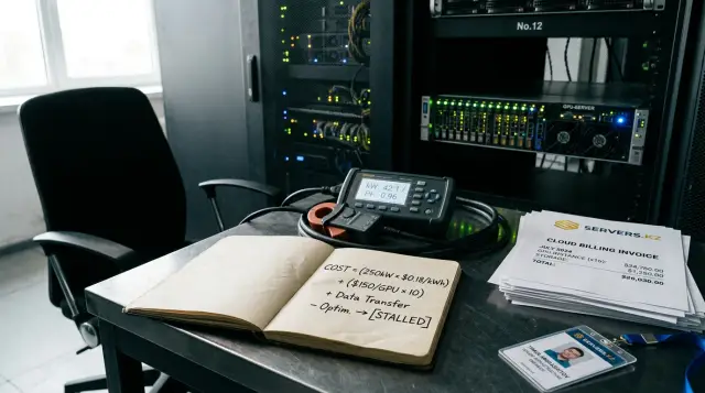
Twenty hours of AI load per week looks like an argument for the cloud: you pay only while the work runs and do not leave an expensive accelerator idle. In practice, the decision depends less on calendar hours than on what counts as an hour, how much data must move, and whether a job can wait for a free resource. One bad assumption can change the result more than a provider discount.

My working conclusion is simple: at a genuine 20 compute hours per week, the cloud usually costs less at the start and often over the full term, provided the data is already there and engineers automatically shut instances down. An on-premises node wins when load grows, data is large or sensitive, transfer delay obstructs the work, and the organization already knows how to run servers. Calculate both cases over the same horizon, then assess constraints that cannot be given a convenient price.

Twenty hours do not determine the winner

Twenty billable GPU hours and twenty hours of availability for the team are different quantities. A cloud meter usually runs while an instance is on, including when a process waits for data, an engineer debugs the environment, or an abandoned notebook computes nothing. An on-premises accelerator remains available all week even if useful work occupies only a small part of that time.

For a first estimate, take 20 hours a week, 52 weeks, and a three-year horizon. That gives 3,120 hours of useful load. It is a baseline, not a billable total. Multiply it by the cloud idle-time factor. If every compute hour includes 15 minutes of setup and waiting, billable time becomes 3,900 hours. Then add concurrency: two jobs that each need a separate GPU for one hour consume two GPU-hours.

Do not compare an on-premises system with an hourly cloud price by dividing the server purchase by 3,120. The server also includes CPUs, memory, storage, networking, warranty, and power headroom. The cloud likewise sells an instance with CPU, RAM, and disks rather than a bare accelerator, while storage, outbound transfer, and public addresses may be billed separately. A comparison is useful only when accelerator memory, performance, numerical precision, and the surrounding environment are comparable.

Queues matter too. If a researcher can submit an overnight job and collect the result in the morning, one local GPU can serve several users. If five specialists need interactive experiments during the same window, the nominal 20 hours quickly becomes a need for several accelerators or a queue whose lost staff time costs more than the hardware.

Measure the actual workload first

Base the decision on telemetry from four to eight representative weeks, not team estimates. Record process duration, GPU utilization, peak video memory, bytes read and written, concurrent runs, and acceptable wait time. Track data preparation and CPU stages separately because their cost does not belong to the GPU.

On a local Linux node, this command provides a basic sample:

nvidia-smi --query-gpu=timestamp,name,utilization.gpu,memory.used,memory.total,power.draw --format=csv -l 60

Its output has this shape:

timestamp, name, utilization.gpu [%], memory.used [MiB], memory.total [MiB], power.draw [W]
2026/07/28 10:00:00.000, GPU model, 87 %, 18432 MiB, 24576 MiB, 286.40 W

Write the result to a file during the pilot and match timestamps to the job log. An average utilization number can mislead: 25 percent may mean steady light work or four hours at full load followed by twelve idle hours. Capacity planning depends more on peak distribution and on the memory without which the job cannot start.

For a cloud pilot, export instance lifetime, machine type, disks, snapshots, and transfer from billing. Compare these records with actual job duration. The gap is paid organizational idle time. If the platform bills by the minute, the formula remains the same and only rounding becomes more accurate.

Do not forecast from the heaviest week, and do not use an average without headroom. Build three profiles instead: normal, peak, and expected growth over the next year. The decision must handle the normal profile economically, the peak profile technically, and growth without a complete architectural replacement.

A local node costs more than its server price

Calculate three-year ownership cost as hardware purchase plus power, cooling, space, administration, maintenance, networking, and expected downtime losses, less residual value. Tax and accounting treatment differs by organization, so keep depreciation and the cost of capital on separate lines instead of hiding them inside a factor.

A working formula is:

TCO_local = purchase + facility + energy + admin + maintenance + downtime + upgrades - residual_value

Calculate power from measured consumption of the whole system at the outlet. If that measurement is not yet available, add average GPU, CPU, memory, and disk use plus power-supply losses, then apply an infrastructure factor for cooling and power distribution. Do not treat the rated maximum as constant consumption: it sizes electrical service but overstates the bill under variable load.

energy = average_system_kW × powered_hours × electricity_price × facility_factor

Here, powered_hours often greatly exceeds 20 hours a week. A server may stay on for remote access, updates, and quick starts. If it can be shut down outside working windows, include startup time and the risk that the team stops doing it. Use the facility's own accounting for its infrastructure factor; an arbitrary attractive number turns the calculation into decoration.

Administration seldom requires a dedicated employee, but it never costs zero. Estimate hours for procurement, acceptance, installation, drivers, images, access control, monitoring, backup, updates, incident investigation, and component replacement. Multiply them by the full labor cost per hour. If an existing team takes the work, the cost still exists because that team gives up other work.

Add compatible spare parts or an agreed repair time. A single accelerator without backup makes for a cheap estimate and a fragile service. Duplicating a whole node for light load also makes little sense; a tested cloud recovery path can cost less.

The cloud bill extends beyond GPU hours

Cloud cost includes instance time, persistent disks, object storage, snapshots, outbound transfer, interzone traffic, public networking, and operating labor. Exact rates change by region, contract, and provider, so enter prices from the organization's current calculator and invoice and record the extraction date.

TCO_cloud = instance_hours + storage + snapshots + egress + interzone + operations + support

Model at least three purchase modes. On-demand pricing sets the upper bound without a commitment. Interruptible capacity costs less, but the job must checkpoint and survive termination. A term commitment lowers the rate yet turns a variable service into an almost fixed payment; compare it with an on-premises purchase and the risk of underuse.

The most common leak is resource lifecycle rather than the rate. Training finishes, a web interface keeps the process alive, and the instance runs until morning. Prevent this with automation: submit compute as a job, set a maximum lifetime, shut idle machines down, and tag resources with an owner and project. A budget alert reports overspend after it starts; a shutdown policy prevents it.

Data transfer needs its own model. Inbound traffic may be inexpensive or unmetered, but retrieving results and repeatedly moving datasets can incur charges. Even free transfer takes time. One terabyte over a 100 Mbps link takes about 22 hours under ideal conditions, and protocol overhead plus competing traffic makes it slower. If a changing multi-terabyte dataset moves every week, the cloud GPU can spend longer waiting than computing.

Storage continues billing after the accelerator stops. Include working disks, source data, dataset versions, checkpoints, logs, and backups. A deletion policy must preserve reproducibility: losing a trained model to save one snapshot often costs more than storing it.

One calculation exposes decision sensitivity

Consider a hypothetical project to see the mechanism, not to obtain a universal price. The organization supplies every monetary value below. The horizon is 36 months, useful load is 20 GPU-hours per week, the billable cloud factor is 1.25, and the local server is powered for 60 hours per week. The task needs one accelerator with sufficient memory, and the same benchmark has confirmed comparable performance.

Fill the table with these inputs:

| Parameter | Local | Cloud | | Purchase and installation | L | 0 | | Billable GPU hours | 0 | 3900 | | Instance rate | 0 | C | | Average system power, kW | P | 0 | | Powered hours | 9360 | 0 | | Electricity per kWh | E | 0 | | Storage and transfer | D_local | D_cloud | | Operating labor | A_local | A_cloud | | Residual value | R | 0 |

The simplified totals are:

local = L + (P × 9360 × E × facility_factor) + D_local + A_local - R
cloud = (3900 × C) + D_cloud + A_cloud

Divide local by 3,120 useful hours to get an effective local hourly cost at the initial load. This is not the marginal price of another hour. After purchase, each additional run up to capacity costs mainly power and operations, so local economics improve quickly as usage rises.

Now find the break-even point. Subtract cloud expenses that do not depend on load from local cost, then divide by the cloud rate adjusted for idle time and by the number of weeks in the horizon. The result approximates useful weekly hours above which local is cheaper. A precise model adds electricity and variable operations to the denominator.

Test sensitivity by changing C, utilization, cloud idle factor, ownership term, and residual value by 20 percent in either direction. If the winner changes after a small shift in one assumption, there is no financial winner. Privacy, provisioning speed, and the team's ability to operate the system should decide.

Privacy changes the set of allowed options

On-premises placement does not automatically secure data, and the cloud does not automatically make it public. The responsibility boundary differs, as do the risks an organization can control. A local server stays under your physical and network control, but it needs access control, logging, encryption, backups, updates, and secure disk disposal.

Classify the data and model first. Determine whether datasets contain personal, medical, or financial information, state secrets, trade secrets, or material that a contract forbids sending to a third party. Then document permitted processing territories, operators, logging requirements, retention periods, and deletion procedure. Legal and security staff must confirm the list before upload, not after the first invoice.

For cloud use, demand specific answers: where data and backups reside, who can receive administrative access, how keys are managed, where diagnostic logs go, whether the service retains prompts, how media is erased, and whether deletion can be proved. Terms for a managed AI service may differ from those for a plain virtual machine. Do not transfer one product's promise to another.

Ask equally uncomfortable questions of the local node. Does it use individual accounts, least privilege, network segmentation, and access logs? Are disks encrypted, where are keys held, and has backup restoration been tested? Can a contractor remove a replaced drive? A server under a desk with no asset control is often weaker than a properly configured cloud.

If policy prohibits external transfer of a dataset, the cloud price for that job is not infinite; the option is simply disallowed. You might de-identify or aggregate data, train locally, and use the cloud for permitted material. The preparation and review still belong in the cost model.

Operations matter as much as procurement

A local GPU requires compatible drivers, libraries, containers, and firmware. An update for one team can break another team's environment, while an old pinned version eventually obstructs security and support. You need a tested base image, change log, quotas, job queue, temperature and memory-error monitoring, and a named service owner.

The cloud removes hardware repair but not image, permission, and spending management. The team must limit allowed instance types, separate production and experimental accounts, keep infrastructure as configuration, and test recovery. The ability to create a powerful machine in a minute accelerates useful work and overspending equally well.

Compare provisioning time. Local procurement, acceptance, and commissioning may take weeks, after which each run is immediately available. The cloud starts quickly while the required region has quota and capacity. Scarcity of a chosen accelerator, a limit review, or internal approval can disrupt urgent work, so a pilot must test the actual launch path instead of a marketing page.

Define failure in advance. Locally, it can be an accelerator, disk, power, or cooling failure; in the cloud, it can be unavailable capacity, an account error, a network break, or an interruptible instance stopping. Set acceptable recovery time and the cost of delay. If the 20 hours belong to a rare but critical weekly window, average utilization says almost nothing about required reliability.

GSE.kz designs and integrates AI and data-center infrastructure, so the local option can be evaluated as a complete service with delivery and support instead of a loose accelerator board. This does not replace calculation: the request to a supplier must include load profile, memory needs, redundancy, repair time, and growth.

A hybrid design needs a clear boundary

A hybrid option often controls risk best: steady sensitive jobs run locally, while rare peaks or experiments use the cloud. Yet two environments create two access systems, two sets of images, and a new data-transfer path. Without a defined boundary, hybrid soon becomes the most expensive choice.

Split work by properties, not by team preference. Keep datasets that cannot leave, predictable repeated jobs, and processes obstructed by network delay on premises. Send temporary experiments, peak queues, jobs needing a rare accelerator, and de-identified datasets to the cloud if contract and policy permit it.

Make portability testable. One container or reproducible image should run a test dataset in both environments; driver versions can differ, but application dependencies stay pinned. Keep a small permitted test dataset and expected result. Run the recovery route each quarter, or it probably will not work on the day of a failure.

Do not promise transparent movement of multi-terabyte datasets. Name the system holding the primary copy, define permitted derived data, and count every synchronization. Sending compute to data sometimes costs less than sending data to compute. Turn that sentence into a routing rule instead of leaving it as an architecture slogan.

Before procurement, request a configuration breakdown rather than one total price. It should list each accelerator's model and memory, available PCIe lanes, CPU memory, network throughput, drive type and endurance, power supplies, warranty terms, and replacement time. Two servers with the same GPU behave differently when one cannot feed data or write checkpoints quickly enough. The detail also prevents comparison of a complete local server with a cloud instance that lacks persistent storage and backup.

The validation benchmark must reflect production work. A short synthetic test can find an obvious cooling or driver fault but predicts training on your dataset poorly. Use a typical model, one heavy case, the real data pipeline, and required precision. Run several trials after warm-up and save the command, environment versions, duration, peak memory, and output size. If a supplier or internal team cannot reproduce it, the performance number does not belong in the financial model.

Price queueing carefully. Do not call every wait hour a lost employee hour, since many jobs run overnight without blocking anyone. Record only delays that stopped the specialist from continuing an experiment, missed a release window, or forced lower-priority work. Those delays during the pilot produce a more honest capacity-shortage cost. It may justify a second local accelerator, cloud bursting, or scheduling, but it does not automatically justify the most expensive option.

Treat useful life differently for equipment and workload. A server may run physically for five years even though a new project needs more video memory or another compute format after three. Residual value then depends on real secondary use inside the organization, not an accounting entry. If the old node can serve inference, visualization, or a teaching environment, it has a defined use. If nobody wants it, do not invent a high residual value to improve payback.

Separate reversible and irreversible choices in the cloud model too. An on-demand instance is easy to replace, but data migration, managed-service dependence, and a long-term discount can bind the architecture more tightly than a purchased server. Estimate exit cost: data retrieval, image conversion, result revalidation, and engineering time. It need not all be added to the base case. Show it as a separate scenario so decision-makers can see the price of changing direction.

The financial sheet must preserve the origin of every number. Put a source and date beside a rate, a role and hours beside labor, a measurement method beside power, and the forecast owner beside growth. Then disagreements do not revolve around the last row: anyone can replace a disputed assumption and see the result. A range is more honest than false precision to the last unit of currency while delivery time, exchange rates, and future load remain unknown.

Finally, agree on who decides when criteria conflict. The budget owner sets the horizon and cost of capital, security defines allowed data, engineering owns the measured profile and operations, and the business owner prices waiting. One person approves the outcome and review date. Otherwise, different people compare cloud and local systems with different premises, and the most persuasive slide wins instead of the suitable infrastructure.

Keep the pilot record with the calculation. State the input dataset, model hash or version, launch command, start and finish time, accelerator type, memory use, output size, and every manual pause. Repeat one run at another time of day to expose effects from shared networking and neighboring jobs. Attach the billing line for the cloud and a power measurement over the same interval for the local node. This record needs no elaborate observability system, yet six months later it explains exactly why those factors entered the sheet. Without it, a new engineer must prove every initial premise again or trust numbers whose origin nobody remembers.

The decision must pass a pilot and a financial threshold

At 20 hours a week, begin with a short cloud pilot if policy permits the data and the team lacks a suitable node. The pilot reveals memory, actual duration, idle time, transfer volume, and environment needs without an irreversible purchase. Limit both budget and resource lifetime before the first run.

After the pilot, complete both 36-month models and test sensitivity. A local purchase is justified by one of three results: its TCO stays lower over a defensible range of assumptions; external transfer is prohibited; or delay, availability, and data volume make the cloud process unacceptable. Without one of these findings, hardware becomes an expensive way to avoid cloud spending discipline.

The reverse error is also common. An organization pays on demand for a stable workload for years because procurement seems difficult. When telemetry shows a persistent queue, a high paid-idle factor, or regular large transfers, recalculate local and committed cloud capacity. A past decision need not remain correct after growth.

Set the review trigger in advance, such as useful GPU-hours per week, queue length, monthly transfer, or resource wait time. A financial sheet without a trigger becomes obsolete silently. A good decision does not guess the next three years of prices; it states which change requires opening the calculation again.